Object - Mock rnaseq • HTRfit

library(HTRfit)

In this section, you will explore how to generate RNAseq data based on the list var object. The mock_rnaseq() function enables you to manage parameters in your RNAseq design, including number of genes, minimum and maximum number of replicates within your experimental setup, sequencing depth, basal expression of each gene, and dispersion of gene expression used for simulating counts.

In addition, we will introduce how to generate complex RNAseq design with diverse gene behaviors by combining several mock_obj into a single one.

Minimal example

list_var <- init_variable( name = "varA", sd = 0.2, level = 2) %>%
            init_variable( name = "varB", sd = 0.43, level = 2) %>%
            add_interaction( between_var = c("varA", "varB"), sd = 0.2)

## -- Required parameters
N_GENES = 6000
MIN_REPLICATES = 2
MAX_REPLICATES = 10
########################

## -- simulate RNAseq data based on list_var, minimum input required
## -- number of replicate randomly defined between MIN_REP and MAX_REP
mock_data <- mock_rnaseq(list_var, N_GENES,
                         min_replicates  = MIN_REPLICATES,
                         max_replicates = MAX_REPLICATES)

## -- simulate RNAseq data based on list_var, minimum input required
## -- Same number of replicates between conditions
mock_data <- mock_rnaseq(list_var, N_GENES,
                         min_replicates  = MAX_REPLICATES,
                         max_replicates = MAX_REPLICATES)

Scaling genes counts based on sequencing depth

Sequencing depth is a critical parameter affecting the statistical power of an RNAseq analysis. With the sequencing_depth option in the mock_rnaseq() function, you have the ability to control this parameter.

## -- Required parameters
N_GENES = 6000
MIN_REPLICATES = 2
MAX_REPLICATES = 10
########################

SEQ_DEPTH = c(100000, 5000000, 10000000)## -- Possible number of reads/sample
SEQ_DEPTH =  10000000 ## -- all samples have same number of reads
mock_data <- mock_rnaseq(list_var, N_GENES,
                         min_replicates  = MIN_REPLICATES,
                         max_replicates = MAX_REPLICATES,
                         sequencing_depth = SEQ_DEPTH)

Set dispersion of gene expression

The dispersion parameter (\(alpha_i\)), characterizes the relationship between the variance of the observed read counts and its mean value. In simple terms, it quantifies how much we expect observed counts to deviate from the mean value. You can specify the dispersion for individual genes using the dispersion parameter.


## -- Required parameters
N_GENES = 6000
MIN_REPLICATES = 2
MAX_REPLICATES = 4
########################

DISP = 0.1 ## -- Same dispersion for each genes
DISP = 1000 ## -- Same dispersion for each genes
DISP = runif(N_GENES, 0, 1000) ## -- Dispersion can vary between genes
mock_data <- mock_rnaseq(list_var, N_GENES,
                         min_replicates  = MIN_REPLICATES,
                         max_replicates = MAX_REPLICATES,
                         dispersion = DISP  )

Set basal gene expression

The basal gene expression parameter, defined using the basal_expression option, allows you to control the fundamental baseline of expression level of genes. When a single value is specified, the basal expression of all genes is the same and the effects of variables defined in list_var are applied from this basal expression level. When several values are specified, the basal expression of each gene is picked randomly among these values (with replacement). The effects of variables are then applied from the basal expression of each gene. This represents the fact that expression levels can vary among genes even when not considering the effects of the defined variables (for example, some genes are constitutively more highly expressed than others because they have stronger basal promoters).

## -- Required parameters
N_GENES = 6000
MIN_REPLICATES = 10
MAX_REPLICATES = 10
########################

BASAL_EXPR = -3 ## -- Value can be negative to simulate low expressed gene
BASAL_EXPR = 2 ## -- Same basal gene expression for the N_GENES
BASAL_EXPR = c( -3, -1, 2, 8, 9, 10 ) ## -- Basal expression can vary between genes
mock_data <- mock_rnaseq(list_var, N_GENES,
                         min_replicates  = MIN_REPLICATES,
                         max_replicates = MAX_REPLICATES,
                         basal_expression = BASAL_EXPR)

Mock RNAseq object

str(mock_data, max.level = 1)
#> List of 6
#>  $ settings       :'data.frame': 4 obs. of  2 variables:
#>  $ init           :List of 3
#>  $ groundTruth    :List of 2
#>  $ counts         :'data.frame': 6000 obs. of  40 variables:
#>  $ metadata       :'data.frame': 40 obs. of  3 variables:
#>   ..- attr(*, "out.attrs")=List of 2
#>  $ scaling_factors: NULL

Combine mock rnaseq object

To generate complex biological experiments with diverse gene behaviors, the combine_mock() function offers the capability to merge multiple mock RNAseq objects.

N_GENES <- 50
REP_NB <- 4
SEQ_DEPTH = c(100000, 5000000, 10000000)## -- Possible number of reads/sample
BASAL_EXPR = c(2, 3, 4) 
DISP = runif(N_GENES, 0, 1000) ## -- Dispersion can vary between genes
LIST_SD <- c(0.01, 0.04 , 0.07, 0.1, 0.13)

list_mock <- list()
for (SD in LIST_SD) {
  input_var_list <- init_variable(name = "varA", sd = SD, level = 150) %>%
    init_variable(name = "varB", sd = SD, level = 20) %>%
    add_interaction(between_var = c("varA", "varB"), sd =  SD)
  
  ## Use generate_counts = FALSE 
  ## to save computing time and avoid generating something useless
  mock_data <- mock_rnaseq(
                  input_var_list,
                  n_genes = N_GENES/length(LIST_SD),
                  basal_expression = BASAL_EXPR,
                  dispersion = DISP,
                  generate_counts = FALSE) 
  ## append new mock_data in a list
  list_mock <- append(list_mock , list(mock_data))
}

## -- counts are generated with combine_mock from the list_mock obj
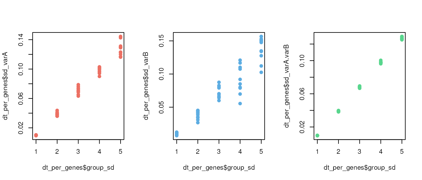
mock_data <- combine_mock(list_mock, REP_NB, REP_NB, SEQ_DEPTH)

The combine_mock() function adds a suffix index to each gene, enabling the attribution of genes to their respective group of origin. By plotting the standard deviation observed after simulation, we can easily differentiate each group of origin.

## -- Compute sd of each variable per genes
dt <- data.table::data.table(subset(mock_data$groundTruth$effects, 
                                    select = c("geneID", "varA", "varB", "varA:varB")))
dt_per_genes <- cbind( dt[ , sd(varA), by = 'geneID' ], 
                       dt[ , sd(varB), by = 'geneID' ]$V1, 
                       dt[ , sd(`varA:varB`), by = 'geneID' ]$V1 )
colnames(dt_per_genes) <- c('geneID', 'sd_varA', 'sd_varB', 'sd_varA.varB')

## suffix of geneID allows for reattribution of gene origin
dt_per_genes$group_sd <- sapply(dt_per_genes$geneID, 
                                           function(x) strsplit(x, "[.]")[[1]][2])

## discriminate group of sd
par(mfrow = c(1, 3))
plot(x = dt_per_genes$group_sd, y = dt_per_genes$sd_varA, col= '#ec7063', pch = 19) # red
plot(x = dt_per_genes$group_sd, y = dt_per_genes$sd_varB, col = '#5dade2', pch = 19) # blue
plot(x = dt_per_genes$group_sd, y = dt_per_genes$sd_varA.varB, col= '#58d68d', pch = 19) # green