Not only RNA-seq
07-rnaseq_notOnly.RmdIn the realm of RNA-seq analysis, it’s widely acknowledged that
counts follow a Negative Binomial distribution. Hence, we recommend
employing family = glmmTMB::nbinom2(link = "log") in the
parameters of fitModelParallel() to align with this
distribution. In RNA-seq it is well known that counts have a Negative
binomial distribution that’s why we recommand using
family = glmmTMB::nbinom2(link = "log") in
fitModelParallel() parameters.
pub_data_fn <- system.file("extdata", "pub_data_rna.tsv", package = "HTRfit")
pub_data <- read.table(file = pub_data_fn, header = TRUE)
plot(density(unlist(round(pub_data[,-1]))), log='x',
              main = "Density of RNA-seq counts")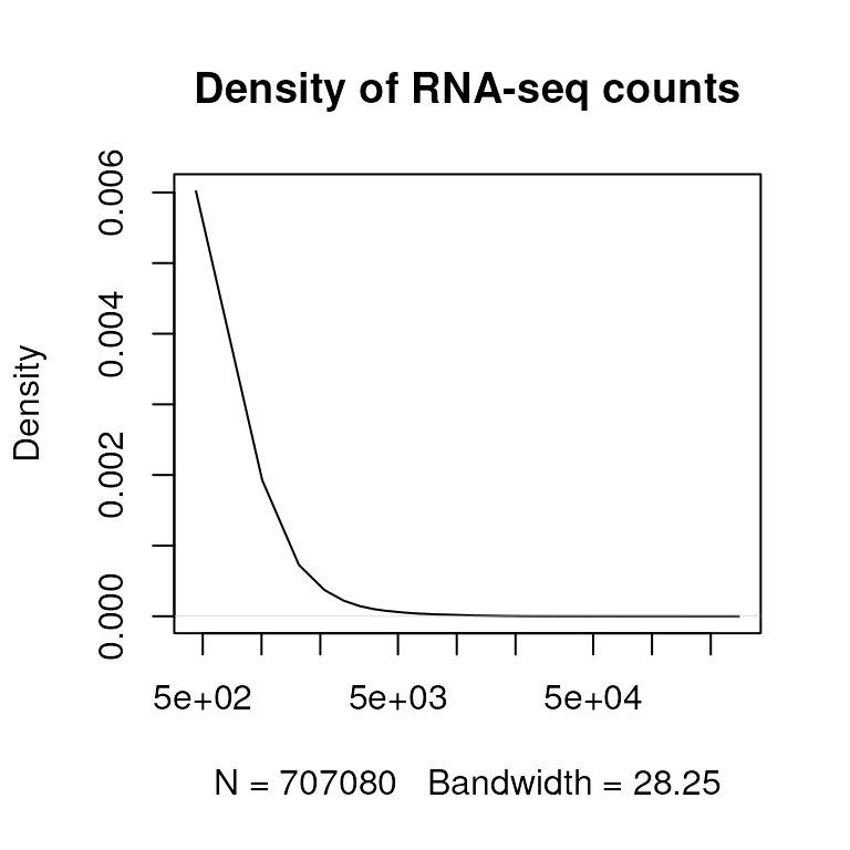
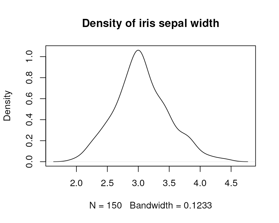
While HTRfit is optimized for RNA-seq data, it’s worth noting that the model family can be customized to accommodate other data types. In a different context, the model family can be adapted according to the nature of your response data. To illustrate, consider an attempt to model Iris sepal length based on sepal width using the iris dataframe. Evaluating the distribution shape of the variable to be modeled (Sepal.Width), we observe a normal distribution.
Given this observation, we opt to fit a model for each species using a Gaussian family model (default). Details about model family here.
l_tmb_iris <- fitModelParallel(
                formula =  Sepal.Width ~ Sepal.Length ,
                data = iris,
                group_by = "Species",
                family = stats::gaussian(),
                n.cores = 1)