Simulation tutorial
02-tutorial.RmdIn this documentation, we will use HTRfit to simulate various experimental design involving multiple experimental condition. To do so, we will first need to estimate plausible parameter values based on publicly available data.
Infering parameters from public data
In this section, we utilize publicly available RNA-seq data from Vande Zande et al. (2022) to estimate parameters for simulating experimental designs using HTRfit. The dataset comprises read counts for 6428 transcripts (genes) among 30 genotypes with 2-4 replicates per genotype.
## -- public data embedded in HTRfit
pub_data_fn <- system.file("extdata", "pub_data_rna.tsv", package = "HTRfit")
pub_data <- read.table(file = pub_data_fn, header = TRUE)
pub_metadata_fn <- system.file("extdata", "pub_metadata.tsv", package = "HTRfit")
pub_metadata <- read.table(file = pub_metadata_fn,  header = TRUE)
Key statistics about the dataset include:
| genes | samples | genotypes | average reads/sample | |
|---|---|---|---|---|
| GSE175398 | 6428 | 111 | 30 | 6852120 |
Model fitting on GSE175398 project RNA-seq dataset
We fit a generalized linear model (GLM) to the data to estimate
plausible parameter distributions. The GLM allows us to estimate
coefficients necessary for simulating experimental conditions. The
tidy_pub_fit object contains HTRfit’s estimates for each
coefficient and gene.
# -- prepare data
## apply + 1 to each counts
## remove genes i with all(k_ij) < 10
data2fit = prepareData2fit(countMatrix = pub_data,
                           metadata = pub_metadata,
                           normalization = 'MRN',
                           response_name = "kij",
                           transform = "x+1",
                           row_threshold = 10)
## --  fit a model
l_tmb <- fitModelParallel(
          formula = kij ~ genotype,
          data = data2fit,
          group_by = "geneID",
          family = glmmTMB::nbinom2(link = "log"),
          n.cores = 8)
## -- remove genes with very low AIC
l_genes <- identifyTopFit(l_tmb)
## -- extract results for best genes
tidy_pub_fit <- tidy_results(l_tmb[l_genes])

## Intercept ~= Basal expr
idx_intercept <- tidy_pub_fit$term == '(Intercept)'
PUB_BASAL_EXPR <- tidy_pub_fit[ idx_intercept , 'estimate' ]
## sd(Beta genotype) = 0.2345902
MAD_OBSERVED <- mad(tidy_pub_fit[ !idx_intercept , 'estimate' ])
## -- dispersion
DISP_PUB  <- glance_tmb(l_tmb)$dispersion
We computed the median absolute deviation (mad) of genotype effects estimated by the model as an estimation of variability robust to outliers.
First simulation: mimicking public data
To implement the experimental setup of the GSE175398
project in our simulation, we initialize 30 levels of genotypes using
the init_variable() function. The estimated intercept
values obtained from analyses of public data shown above correspond to
basal expression levels for each gene in our simulated dataset.
Moreover, we use values of gene dispersion estimated from public data
for our simulation. To simplify the example, only 100 genes are
simulated. Consequently, the value of sequencing depth used in
simulations was obtained by dividing the sequencing depth observed in
public data mean(colSums(pub_data)) by the ratio of the
number of genes in public data (6428) and the number of genes in our
simulation (100).
## -- design to simulate
N_GENES <- 100
MIN_REPLICATES <- 2
MAX_REPLICATES <- 4
SEQ_DEPTH <- mean(colSums(pub_data))/(6428/100)

## -- init effects to simulate
input_var_list <- init_variable( name = "genotype", sd = MAD_OBSERVED, level = 30)
## -- simulate RNA-seq data to mimic public data
mock_data <- mock_rnaseq(input_var_list,
                         n_genes = N_GENES,
                         min_replicates  = MIN_REPLICATES,
                         max_replicates = MAX_REPLICATES,
                         basal_expression = PUB_BASAL_EXPR,
                         sequencing_depth = SEQ_DEPTH,
                         dispersion = DISP_PUB )
Simulated genotype effects are drawn from a normal distribution with
mean = 0 and sd = MAD_OBSERVED. Note that for
a normal distribution, standard deviation (sd) and median absolute
deviation (mad) are equal.
First fit with single fixed effect
We fit a model to the simulated RNA-seq data using the
fitModelParallel() function to estimate for each gene 30
coefficients corresponding to genotype effects.
## -- prepare data simulated to fit
## apply + 1 to each counts
## remove genes i with all(k_ij) < 10
data2fit = prepareData2fit(countMatrix = mock_data$counts,
                           metadata =  mock_data$metadata,
                           normalization = 'MRN',
                           response_name = "kij",
                           transform = "x+1",
                           row_threshold = 10)
## -- fit a model to the simulated data
l_tmb <- fitModelParallel(
          formula = kij ~ genotype,
          data = data2fit,
          group_by = "geneID",
          family = glmmTMB::nbinom2(link = "log"),
          n.cores = 1,
          control = glmmTMB::glmmTMBControl(optCtrl=list(iter.max=1e5,
                                                         eval.max=1e5)))
First evaluation: comparing simulation and fit
Next, we evaluate the perfomance of the model using
evaluation_report() that compares coefficients from
mock_rnaseq() simulations to model’s estimates obtained
with fitModelParallel().
## -- eval params for Wald test
ln_FC_threshold <- log(1.25) ## 25% of expression change
alternative_hypothesis <- "greaterAbs"
## -- remove genes with very low AIC
l_genes <- identifyTopFit(l_tmb)
## -- evaluation
resSimu <- evaluation_report( list_tmb = l_tmb,
                              list_gene = l_genes,
                              mock_obj = mock_data,
                              coeff_threshold = ln_FC_threshold,
                              alt_hypothesis = alternative_hypothesis )
Explore evaluation results - Identity plot
The evaluation_report() function produces an identity
plot, offering a visual tool to juxtapose the simulated effects (actual
effects) with the model-inferred effects. This graphical representation
simplifies assessing how well the model aligns with the values of the
simulated effects, enabling a visual analysis of the model’s goodness of
fit to the simulated data. For a more quantitative evaluation of
inference quality, the R-squared (R^2) and RMSE metrics are also
shown.
## -- Model params
resSimu$identity$params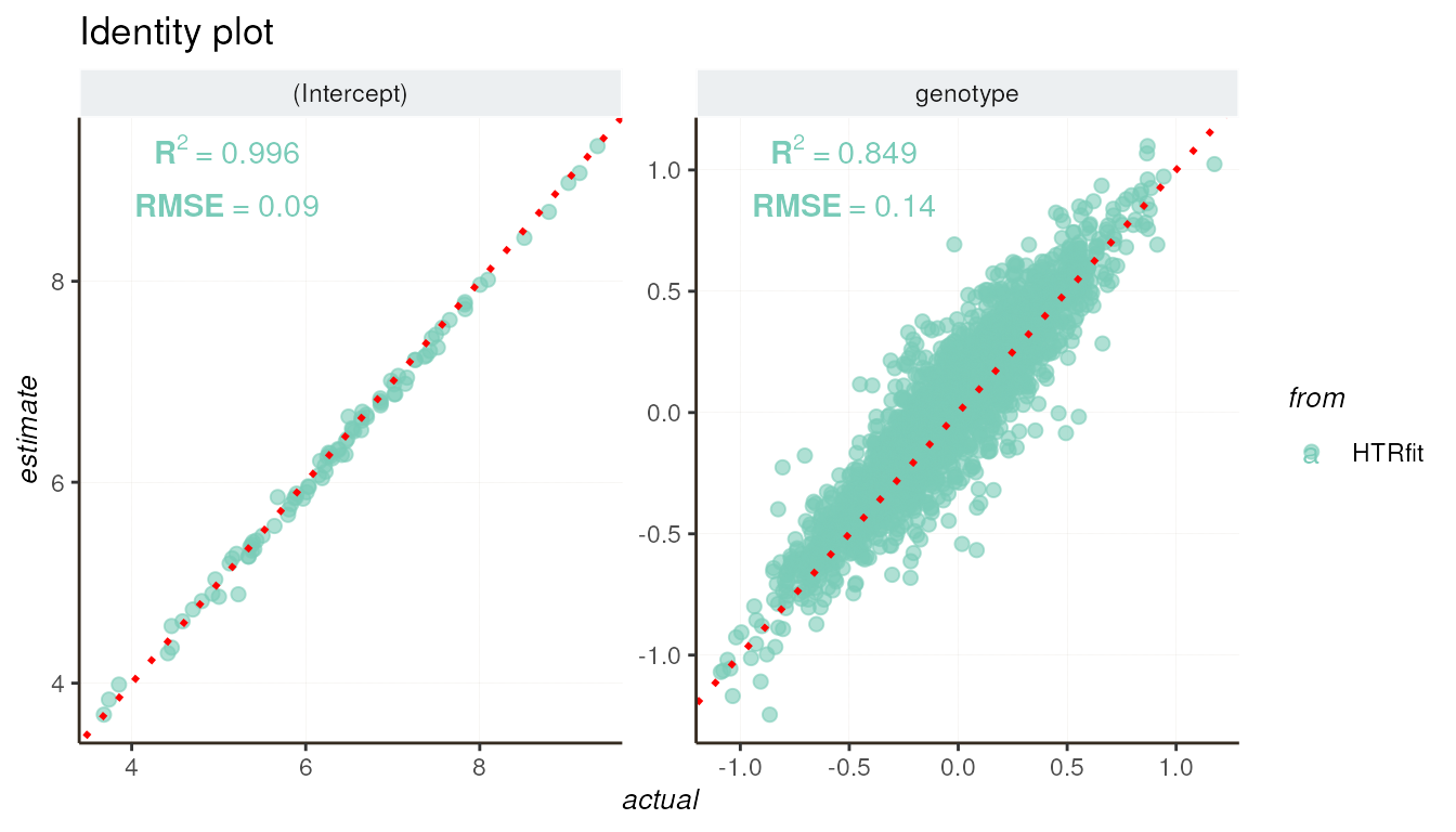
## -- actual/estimate comparison
resSimu$performances$byparams[3, c('description','R2','RMSE')]| description | R2 | RMSE |
|---|---|---|
| genotype | 0.8490975 | 0.1402235 |
Explore evaluation results - ROC curve
The Receiver Operating Characteristic (ROC) curve is a valuable tool
for assessing the performance of classification models, particularly in
the context of identifying differentially expressed genes. It provides a
graphical representation of the model’s ability to distinguish between
genes that are differentially expressed and those that are not, by
varying the coeff_threshold and the
alt_hypothesis parameters.
## -- ROC curve
resSimu$roc$params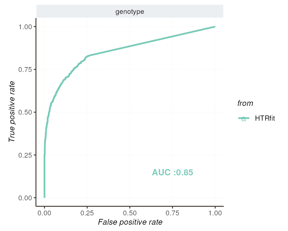
Explore evaluation results - Precision-recall curve
The precision-recall curve (PR curve) illustrates the relationship between precision and recall at various classification thresholds. It is particularly valuable in the context of imbalanced data, where one class is significantly more prevalent than the other. Unlike the ROC curve, which can be influenced by class distribution, the PR curve focuses on the model’s ability to correctly identify examples of the minority class while maintaining high precision.
## -- precision recall by params
resSimu$precision_recall$params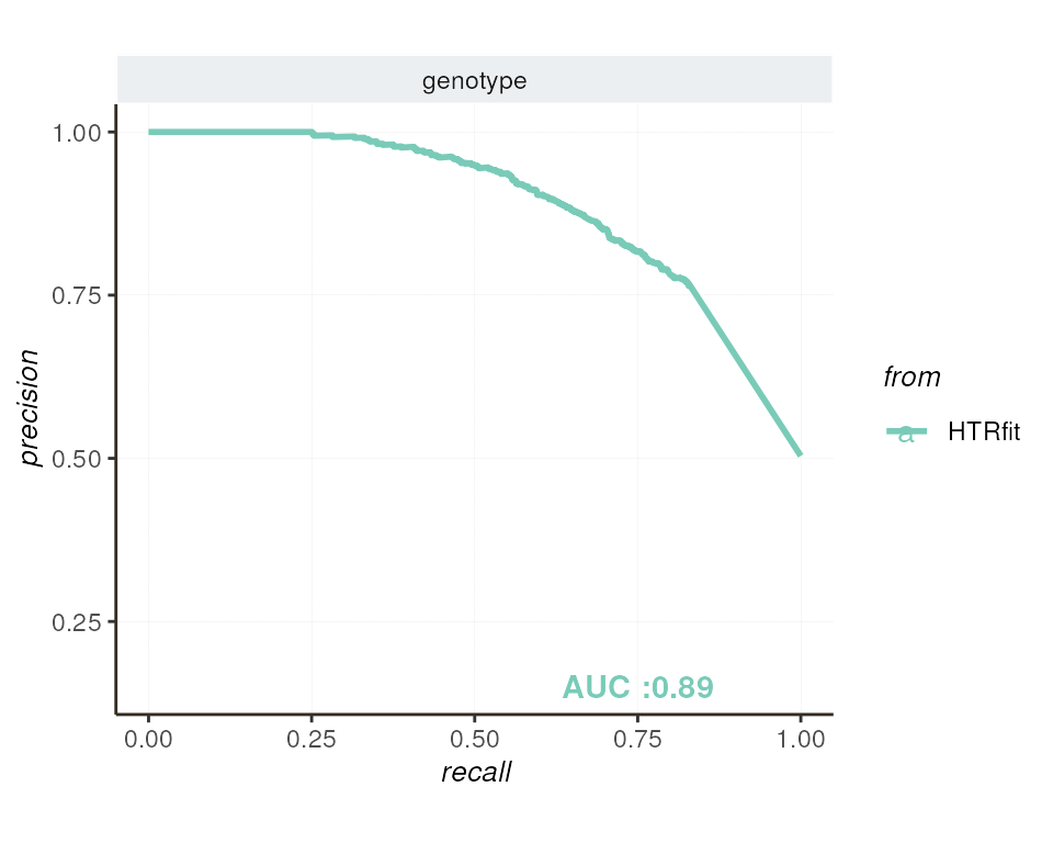
Explore evaluation results - classification metrics
The area under the ROC or PR curve (AUC) provides a single metric
that summarizes the model’s overall performance in distinguishing
between differentially expressed and non-differentially expressed genes.
A higher AUC indicates better model performance. In the case of the ROC
curve, this AUC should be compared to the value of 0.5 corresponding to
the expected AUC for a random classifier. For the PR curve, the random
expectation pr_randm_AUC corresponds to the actual
proportion of differentially expressed genes, which can take any value
between 0 and 1.
The classification metrics are computed for each fixed parameters
(excluding the intercept when
skip_eval_intercept = TRUE).
## -- classification metrics
resSimu$performances$byparams[3, c('description',   'pr_AUC',
                                   'pr_randm_AUC', 'pr_performance_ratio',
'roc_AUC', 'roc_randm_AUC')]| description | pr_AUC | pr_randm_AUC | pr_performance_ratio | roc_AUC | roc_randm_AUC |
|---|---|---|---|---|---|
| genotype | 0.888071 | 0.5036684 | 1.763206 | 0.8527017 | 0.5 |
Fitting and evaluating random effect
In this section, we delve into the process of estimating the standard
deviation of genotype effects (sd(genotype)) using random
effects in HTRfit. By treating genotype as a random effect
(kij ~ (1 | genotype)), HTRfit provides estimates for both
the (Intercept) and sd_(Intercept) for each
gene.
## fit genotype as random effect
l_tmb <- fitModelParallel(
formula = kij ~ (1 | genotype),
data = data2fit,
group_by = "geneID",
family = glmmTMB::nbinom2(link = "log"),
n.cores = 1,
control = glmmTMB::glmmTMBControl(optCtrl=list(iter.max=1e5,
eval.max=1e5)))
## -- eval params for Wald test
ln_FC_threshold <- log(1.25) ## 25% of expression change
alternative_hypothesis <- "greaterAbs"
## -- remove genes with very low AIC
l_genes <- identifyTopFit(l_tmb)
## -- evaluation
resSimu <- evaluation_report( list_tmb = l_tmb,
list_gene = l_genes,
mock_obj = mock_data,
coeff_threshold = ln_FC_threshold,
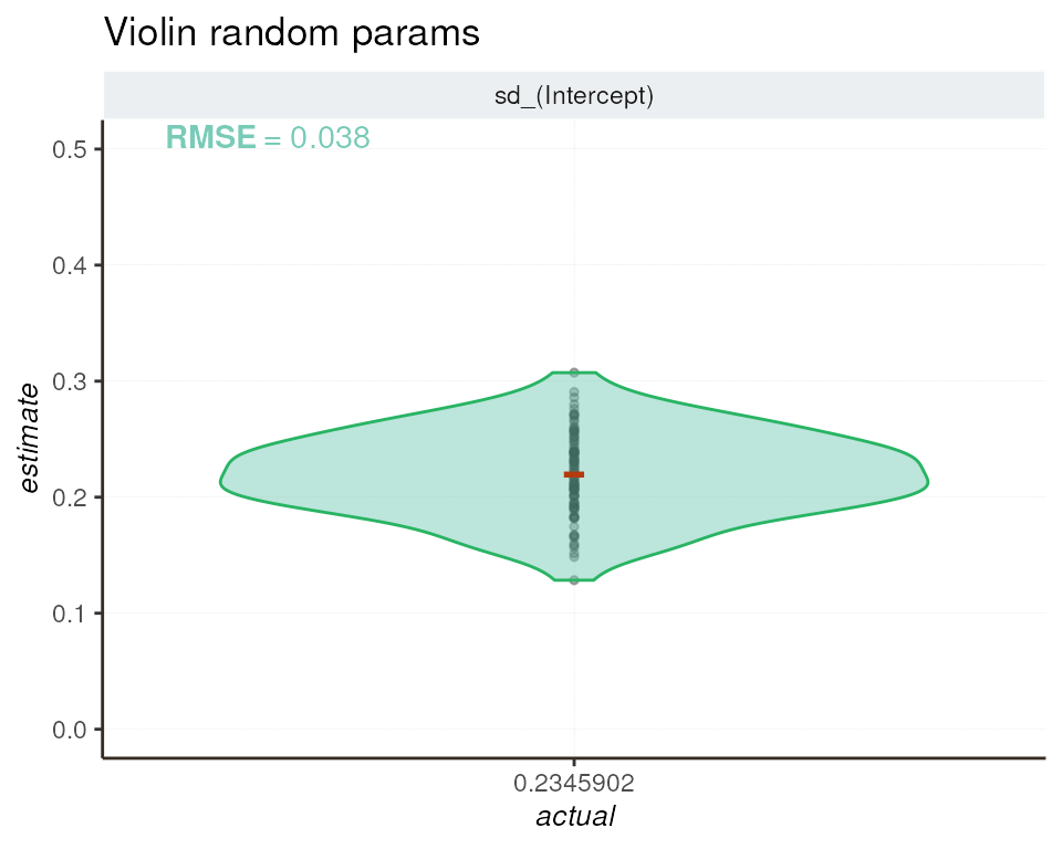
alt_hypothesis = alternative_hypothesis )Explore evaluation results - Violin plot
To evaluate the consistency between estimated and actual values of
the random effect, we employ a violin plot. This graphical
representation showcases how well the sd_(Intercept)
estimates align with the simulated sd(genotype) value
(MAD_OBSERVED = 0.2345902) across genes.
Improving estimation of random effects with additional levels
One approach to improve the estimation of sd(genotype)
involves increasing the number of genotype levels. By expanding the
number of genotype levels in the simulated data, the model has more
power for capturing the inherent variability in genotype effects.
Here, the number of genotype levels is increased from 30 to 300, with
all other paramaters remaining unchanged (sequencing depth, replicates
number, number of genes, basal gene expression).
## -- increase number of level to 300
input_var_list <- init_variable( name = "genotype", sd = MAD_OBSERVED, level = 300)
## -- simulate RNA-seq data
mock_data <- mock_rnaseq(input_var_list,
n_genes = N_GENES,
min_replicates = MIN_REPLICATES,
max_replicates = MAX_REPLICATES,
basal_expression = PUB_BASAL_EXPR,
sequencing_depth = SEQ_DEPTH,
dispersion = DISP_PUB )
## -- prepare data
## apply + 1 to each counts
## remove genes i with all(k_ij) < 10
data2fit = prepareData2fit(countMatrix = mock_data$counts,
metadata = mock_data$metadata,
normalization = 'MRN',
response_name = "kij",
transform = "x+1",
row_threshold = 10)
## fit random effect
l_tmb <- fitModelParallel(
formula = kij ~ (1 | genotype),
data = data2fit,
group_by = "geneID",
family = glmmTMB::nbinom2(link = "log"),
n.cores = 1,
control = glmmTMB::glmmTMBControl(optCtrl=list(iter.max=1e5,
eval.max=1e5)))
## -- eval params for Wald test on fixed
ln_FC_threshold <- log(1.25) ## 25% of expression change
alternative_hypothesis <- "greaterAbs"
## -- remove genes with very low AIC
l_genes <- identifyTopFit(l_tmb)
## -- evaluation
resSimu <- evaluation_report( list_tmb = l_tmb,
list_gene = l_genes,
mock_obj = mock_data,
coeff_threshold = ln_FC_threshold,
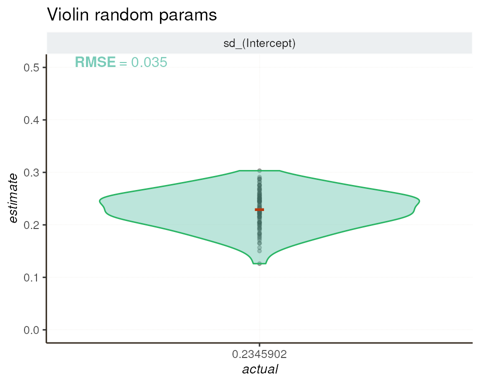
alt_hypothesis = alternative_hypothesis )Following the adjustment in genotype levels, we reevaluate the
model’s performance using the evaluation_report() function.
The resulting violin plot demonstrates the improvement in estimating
sd(genotype), as evidenced by the reduction in RMSE.

It’s important to note that since we only fit random effects, classification metrics are not available in this case (the model cannot estimate the effects of individual genotypes when genotype is treated as a variable with random effects).
Simulating multiple main effects
In this section, we demonstrate how HTRfit can simulate multiple main
effects by “piping” (%>%) the
init_variable() function. To illustrate, we introduce a
second main effect, environment, with two levels. This
allows us to explore the combined effects of genotype and environment on
gene expression. For simplicity, all effects for both variables
(genotype and environment) are drawn from a
normal distribution with mean = 0 and
sd = MAD_OBSERVED (0.2345902). Additionally, we use in our
simulation values of gene dispersion, basal expression, and sequencing
depth obtained from analyses of the public dataset mentioned above. For
faster computation, we simulate data for only 100 genes, adjusting the
sequencing depth accordingly.
N_GENES <- 100
MIN_REPLICATES <- 4
MAX_REPLICATES <- 4
SEQ_DEPTH <- mean(colSums(pub_data))/N_GENES
## -- init design
input_var_list <- init_variable( name = "genotype", sd = MAD_OBSERVED, level = 30) %>%
                  init_variable( name = "environment", sd = MAD_OBSERVED, level = 2 )
## -- simulate RNA-seq data
mock_data <- mock_rnaseq(input_var_list,
                         n_genes = N_GENES,
                         min_replicates  = MIN_REPLICATES,
                         max_replicates = MAX_REPLICATES,
                         basal_expression = PUB_BASAL_EXPR,
                         sequencing_depth = SEQ_DEPTH,
                         dispersion = DISP_PUB )
Fitting and evaluating multiple fixed effects
We fit a model to the simulated RNA-seq data, incorporating both genotype and environment as main effects. Subsequently, we evaluate the model’s performance using metrics and graphical representations available in HTRfit.
## -- prepare data
## apply + 1 to each counts
## remove genes i with all(k_ij) < 10
data2fit = prepareData2fit(countMatrix = mock_data$counts,
                           metadata =  mock_data$metadata,
                           normalization = 'MRN',
                           response_name = "kij",
                           transform = "x+1",
                           row_threshold = 10)
## fit complex model
l_tmb <- fitModelParallel(
          formula = kij ~ genotype + environment,
          data = data2fit,
          group_by = "geneID",
          family = glmmTMB::nbinom2(link = "log"),
          n.cores = 1,
          control = glmmTMB::glmmTMBControl(optCtrl=list(iter.max=1e5,
                                                         eval.max=1e5)))
## -- eval params for Wald test
ln_FC_threshold <- log(1.25) ## 25% of expression change
alternative_hypothesis <- "greaterAbs"
## -- remove genes with very low AIC
l_genes <- identifyTopFit(l_tmb)
## -- evaluation
resSimu <- evaluation_report( list_tmb = l_tmb,
                              list_gene = l_genes,
                              mock_obj = mock_data,
                              coeff_threshold = ln_FC_threshold,
                              alt_hypothesis = alternative_hypothesis )
Explore evaluation results - Identity plot
The identity plot provides a visual tool to assess how well the model aligns with the values of the simulated effects. It enables a straightforward analysis of the model’s goodness of fit to the simulated data.
## -- Model params
resSimu$identity$params
R² and RMSE obtained for each fixed effects are summarized bellow:
## -- actual/estimate comparison
resSimu$performances$byparams[3:4, c('description', 'R2', 'RMSE')]| description | R2 | RMSE |
|---|---|---|
| environment | 0.9911976 | 0.0367530 |
| genotype | 0.9162173 | 0.1186953 |
Explore evaluation results - ROC curve
The Receiver Operating Characteristic (ROC) curve evaluates the model’s ability to distinguish between differentially expressed genes. By varying the classification threshold, this curve offers insights into the model’s discriminatory power.
## -- ROC curve
resSimu$roc$params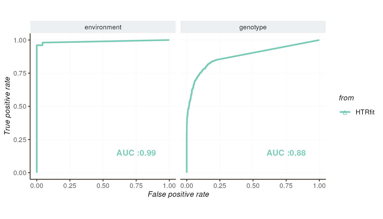
Explore evaluation results - Precision-recall curve
The precision-recall curve illustrates the trade-off between precision and recall at different classification thresholds. Particularly useful for imbalanced datasets, it highlights the model’s ability to correctly identify examples of the minority class while maintaining high precision.
## -- precision recall by params
resSimu$precision_recall$params
Explore evaluation results - Metrics summary
Finally, we summarize the model’s performance using classification metrics.
## -- classification metrics
resSimu$performances$byparams[3:4, c('description', 'pr_AUC',
                                     'pr_randm_AUC', 'pr_performance_ratio',
'roc_AUC', 'roc_randm_AUC')]| description | pr_AUC | pr_randm_AUC | pr_performance_ratio | roc_AUC | roc_randm_AUC |
|---|---|---|---|---|---|
| environment | 0.9942121 | 0.5257732 | 1.890952 | 0.9889173 | 0.5 |
| genotype | 0.9189461 | 0.5264842 | 1.745439 | 0.8807178 | 0.5 |
Fitting and evaluating mixed model
In this section, we utilize a mixed model approach to estimate the
fixed effect of environment and the variability of
genotype effects using HTRfit. By specifying the model
formula as kij ~ environment + (1 | genotype), we obtain
estimates for the fixed effect of environment for each
gene, along with an estimate of the variability of genotype
effects (referred to as sd(Intercept) by the model). The
mixed model incorporates both the fixed effect of
environment and the random effect of genotype,
allowing us to capture the influence of environmental factors on gene
expression while accounting for genotypic variability. We fit this model
to simulated RNA-seq data and evaluate its performance using various
metrics.
## fit complex model
l_tmb <- fitModelParallel(
          formula = kij ~  environment + ( 1 | genotype ) ,
          data = data2fit,
          group_by = "geneID",
          family = glmmTMB::nbinom2(link = "log"),
          n.cores = 1,
          control = glmmTMB::glmmTMBControl(optCtrl=list(iter.max=1e5,
                                                         eval.max=1e5)))
## -- eval params for Wald test
ln_FC_threshold <- log(1.25) ## 25% of expression change
alternative_hypothesis <- "greaterAbs"
## -- remove genes with very low AIC
l_genes <- identifyTopFit(l_tmb)
## -- evaluation
resSimu <- evaluation_report( list_tmb = l_tmb,
                              list_gene = l_genes,
                              mock_obj = mock_data,
                              coeff_threshold = ln_FC_threshold,
                              alt_hypothesis = alternative_hypothesis )
Explore evaluation results - ROC curve
Given the inclusion of a fixed effect (environment), the
ROC curve provides insights into the model’s ability to discriminate
between differentially expressed genes based on environmental factors.
By varying the classification threshold, we assess the model’s
discriminatory power in distinguishing between gene expression
patterns.
## -- ROC curve
resSimu$roc$params
Explore evaluation results - Precision-recall curve
Similarly, the precision-recall curve evaluates the model’s performance in identifying differentially expressed genes across various classification thresholds. This curve offers valuable insights, particularly in scenarios with imbalanced datasets, by highlighting the trade-off between precision and recall.
## -- precision recall by params
resSimu$precision_recall$params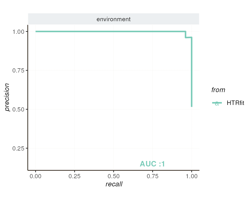
Explore evaluation results - Violin plot
We also visualize the distribution of random parameters estimation.
The violin plot provides a graphical representation of proximity between
the actual sd(genotype) values and their corresponding
estimations provided by the model.
Explore evaluation results - Metrics summary
Finally, we summarize the model’s performance using key metrics, including R-squared (R²) and root mean square error (RMSE) for regression tasks, as well as area under the curve (AUC) for classification tasks.
## -- actual/estimate comparison
resSimu$performances$byparams[3:4, c('description', 'R2', 'RMSE')]| description | R2 | RMSE |
|---|---|---|
| environment | 0.9911375 | 0.0364681 |
| sd_(Intercept) | NA | 0.0354861 |
## -- classification metrics
resSimu$performances$byparams[3, c('description',   'pr_AUC',
                                   'pr_randm_AUC', 'pr_performance_ratio',
'roc_AUC', 'roc_randm_AUC')]| description | pr_AUC | pr_randm_AUC | pr_performance_ratio | roc_AUC | roc_randm_AUC |
|---|---|---|---|---|---|
| environment | 0.9984914 | 0.5151515 | 1.938248 | 0.998366 | 0.5 |
Simulating interactions
HTRfit offers the capability to initialize and simulate complex
experimental designs involving multiple variables with varying numbers
of levels, as well as interactions between main effects of these
variables. To illustrate this capability, let’s simulate an RNA-seq
experiment with 30 genotype levels and 2 environmental conditions. Using
the add_interaction() function, interactions between each
level can also be simulated. For simplicity, main effects and
interaction effects are all drawn from a normal distribution with
mean = 0 and sd = MAD_OBSERVED (0.2345902).
Additionally, we use in our simulation values of gene dispersion, basal
expression, and sequencing depth obtained from analyses of the public
dataset mentioned above. For faster computation, we simulate data for
only 100 genes, adjusting the sequencing depth accordingly.
N_GENES <- 100
MIN_REPLICATES <- 4
MAX_REPLICATES <- 4
SEQ_DEPTH <- mean(colSums(pub_data))/N_GENES

## -- init design
input_var_list <- init_variable( name = "genotype", sd = MAD_OBSERVED, level = 30) %>%
                  init_variable( name = "environment", sd = MAD_OBSERVED, level = 2 ) %>%
                  add_interaction(between_var = c("genotype", "environment"),
                                  sd = MAD_OBSERVED)
## -- simulate RNA-seq data
mock_data <- mock_rnaseq(input_var_list,
                         n_genes = N_GENES,
                         min_replicates  = MIN_REPLICATES,
                         max_replicates = MAX_REPLICATES,
                         basal_expression = PUB_BASAL_EXPR,
                         sequencing_depth = SEQ_DEPTH,
                         dispersion = DISP_PUB )
Fitting and evaluating interaction with fixed model
## -- prepare data
## apply + 1 to each counts
## remove genes i with all(k_ij) < 10
data2fit = prepareData2fit(countMatrix = mock_data$counts,
                           metadata =  mock_data$metadata,
                           normalization = 'MRN',
                           response_name = "kij",
                           transform = "x+1",
                           row_threshold = 10)
## fit complex model
l_tmb <- fitModelParallel(
          formula = kij ~ genotype + environment + genotype:environment,
          data = data2fit,
          group_by = "geneID",
          family = glmmTMB::nbinom2(link = "log"),
          n.cores = 1,
          control = glmmTMB::glmmTMBControl(optCtrl=list(iter.max=1e5,
                                                         eval.max=1e5)))
## -- eval params for Wald test
ln_FC_threshold <- log(1.25) ## 25% of expression change
alternative_hypothesis <- "greaterAbs"
## -- remove genes with very low AIC
l_genes <- identifyTopFit(l_tmb)
## -- evaluation
resSimu <- evaluation_report( list_tmb = l_tmb,
                              list_gene = l_genes,
                              mock_obj = mock_data,
                              coeff_threshold = ln_FC_threshold,
                              alt_hypothesis = alternative_hypothesis )
Identity Plot, ROC Curve, and Precision-Recall Curve
These plots provide visual assessments of how well the model aligns with the values of the simulated effects and its ability to distinguish between differentially expressed genes. Each curve represents a different aspect of the model’s performance, including its goodness of fit and classification accuracy.
## -- Model params
resSimu$identity$params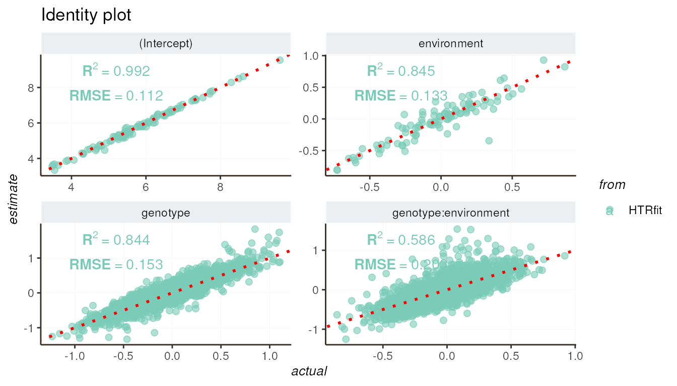
resSimu$performances$byparams[3:5, c('description', 'R2', 'RMSE')]| description | R2 | RMSE |
|---|---|---|
| environment | 0.8452716 | 0.1329940 |
| genotype | 0.8437769 | 0.1530331 |
| genotype:environment | 0.5861132 | 0.2026707 |
## -- ROC curve
resSimu$roc$params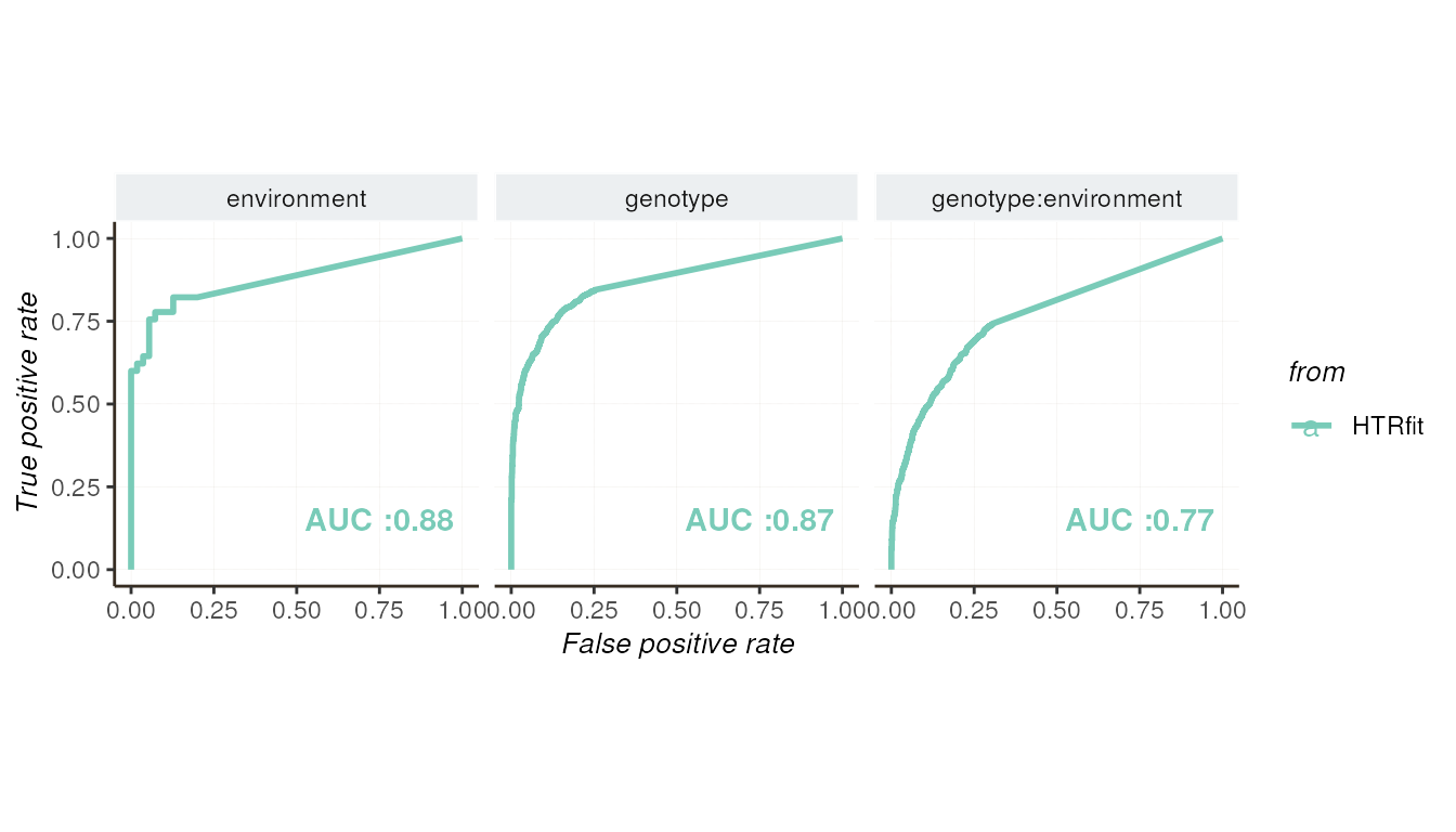
## -- precision recall by params
resSimu$precision_recall$params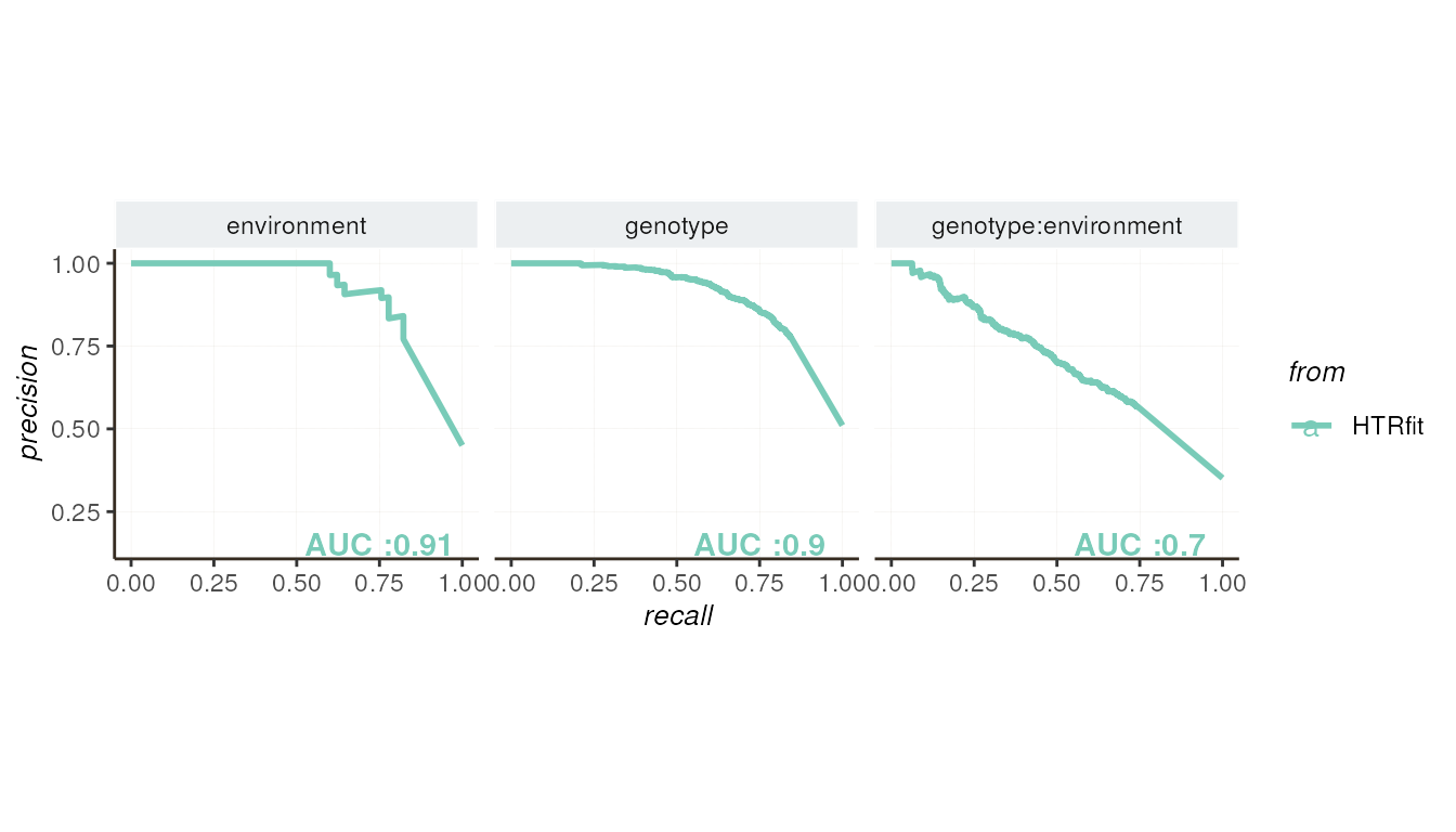
Metrics summary
The following table summarizes the AUC obtained:
resSimu$performances$byparams[3:5, c('description', 'pr_AUC',
                                     'pr_randm_AUC', 'pr_performance_ratio',
'roc_AUC', 'roc_randm_AUC')]| description | pr_AUC | pr_randm_AUC | pr_performance_ratio | roc_AUC | roc_randm_AUC |
|---|---|---|---|---|---|
| environment | 0.9092767 | 0.4500000 | 2.020615 | 0.8787879 | 0.5 |
| genotype | 0.9027545 | 0.5103448 | 1.768911 | 0.8680463 | 0.5 |
| genotype:environment | 0.7046191 | 0.3513793 | 2.005295 | 0.7673864 | 0.5 |
Fitting and evaluating interaction with mixed model
HTRfit can estimate the interaction between a variable with fixed
effects and a variable with random effects using mixed models such as
the following model:
kij ~ environment + ( environment | genotype ). With this
model, HTRfit provides estimates for fixed effect of the
environment for each gene, as well as an estimate of the
standard deviation of genotypic effects (referred to as
sd_(Intercept) by the model) and the standard deviation of
interactions between genotype and environment (referred to as
sd_(environment) by the model).
## fit complex model
l_tmb <- fitModelParallel(
          formula = kij ~  environment + ( environment | genotype ) ,
          data = data2fit,
          group_by = "geneID",
          family = glmmTMB::nbinom2(link = "log"),
          n.cores = 1,
          control = glmmTMB::glmmTMBControl(optCtrl=list(iter.max=1e5,
                                                         eval.max=1e5)))
## -- eval params for Wald test
ln_FC_threshold <- log(1.25) ## 25% of expression change
alternative_hypothesis <- "greaterAbs"
## -- remove genes with very low AIC
l_genes <- identifyTopFit(l_tmb)
## -- evaluation
resSimu <- evaluation_report( list_tmb = l_tmb,
                              list_gene = l_genes,
                              mock_obj = mock_data,
                              coeff_threshold = ln_FC_threshold,
                              alt_hypothesis = alternative_hypothesis )
ROC Curve and Precision-Recall Curve
Both the ROC curve and the precision-recall curve provide insights into the classification performance of the model, particularly regarding its ability to distinguish between differentially expressed genes and non-differentially expressed genes.
## -- ROC curve
resSimu$roc$params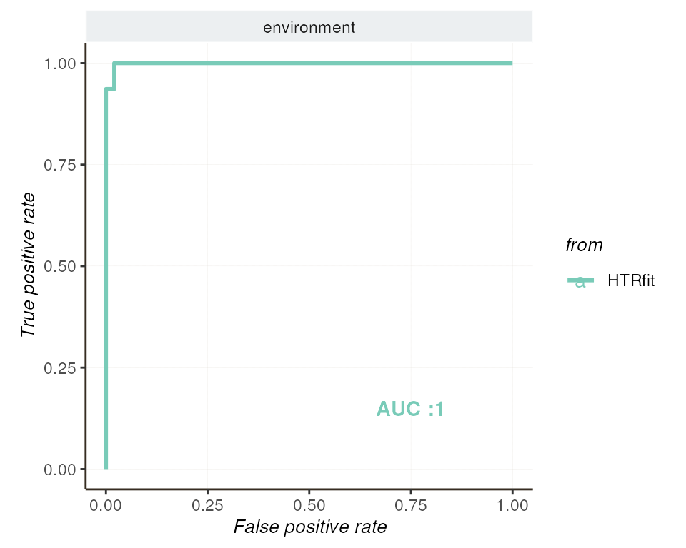
## -- precision recall by params
resSimu$precision_recall$params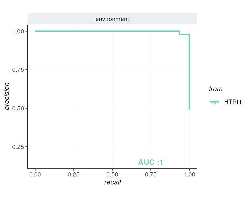
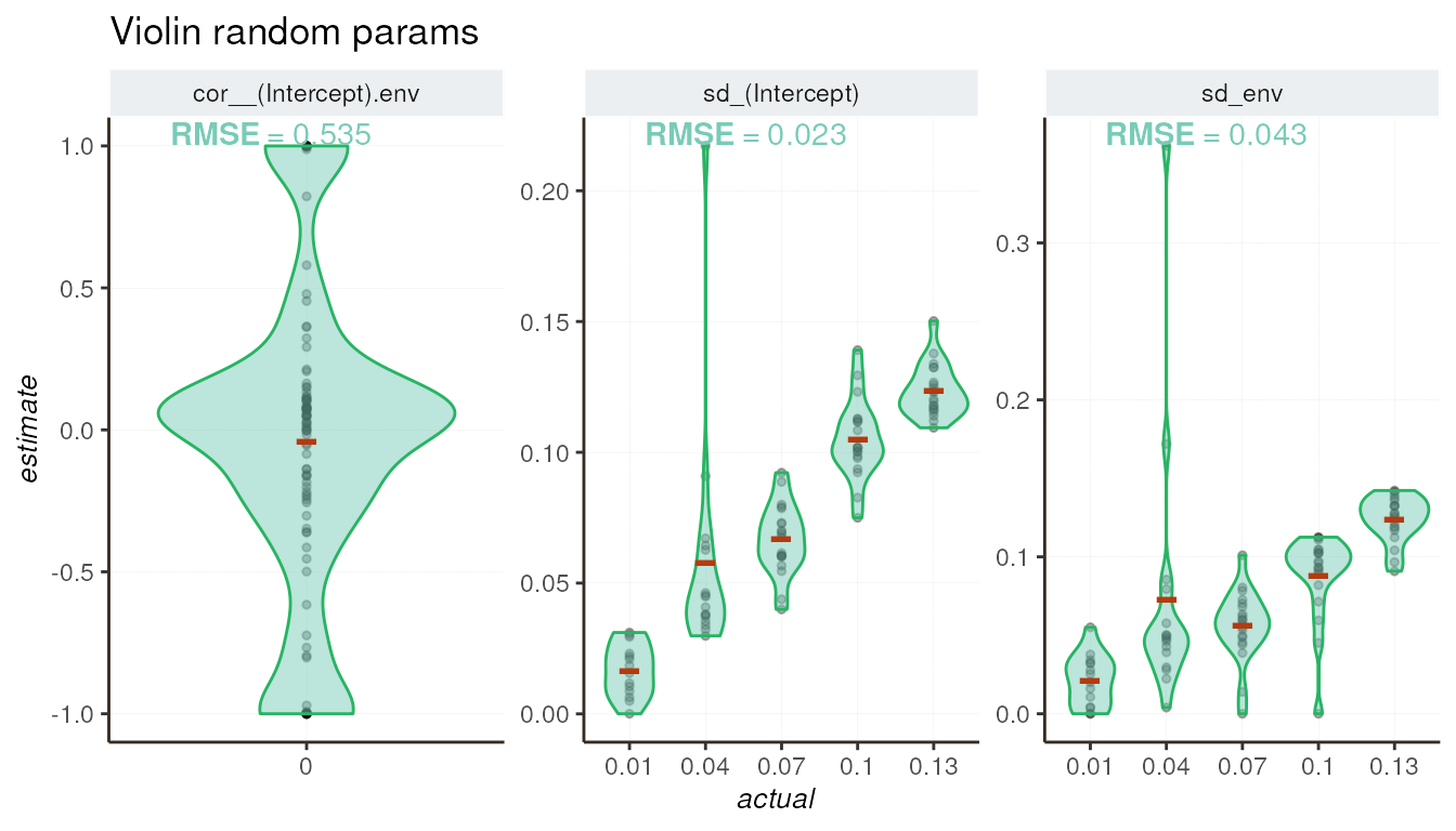
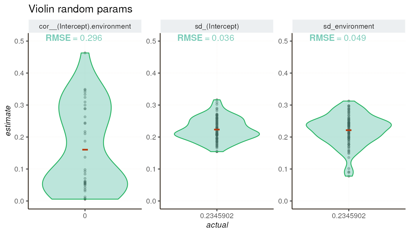
Violin plot for random parameters
The violin plot visualizes the distribution of random parameter
estimates and shows how close these estimates are to the actual values
from simulations. Additionally, the model returns
cor__(Intercept).env, which represents the correlation
between the basal expression of the gene and the environmental effect.
This parameter was always set to 0 in our simulations.
Metrics summary
The following table summarizes the model’s performance metrics, including R-squared (R2), root mean squared error (RMSE), precision-recall area under the curve (PR AUC), and receiver operating characteristic area under the curve (ROC AUC).
## -- actual/estimate comparison
resSimu$performances$byparams[c(2,4,5,6), c('description', 'R2', 'RMSE')]| description | R2 | RMSE |
|---|---|---|
| cor__(Intercept).environment | NA | 0.2956328 |
| environment | 0.9902667 | 0.0354384 |
| sd_(Intercept) | NA | 0.0363083 |
| sd_environment | NA | 0.0488314 |
## -- classification metrics
resSimu$performances$byparams[4, c('description',   'pr_AUC',
                                   'pr_randm_AUC', 'pr_performance_ratio',
'roc_AUC', 'roc_randm_AUC')]| description | pr_AUC | pr_randm_AUC | pr_performance_ratio | roc_AUC | roc_randm_AUC |
|---|---|---|---|---|---|
| environment | 0.9986267 | 0.4895833 | 2.039748 | 0.9986974 | 0.5 |
Simulating, fitting and evaluating triple interaction
HTRfit’s capability extends to simulating triple interactions to
evaluate the model’s performance in capturing such complex
relationships. To demonstrate this, we introduce a categorical variable
age to investigate how RNA levels vary with the age of
organisms. We initialize this variable with three levels.
N_GENES <- 100
MIN_REPLICATES <- 4
MAX_REPLICATES <- 4
SEQ_DEPTH <- mean(colSums(pub_data))/N_GENES
## -- init design
input_var_list <- init_variable( name = "genotype", sd = MAD_OBSERVED, level = 30) %>%
                  init_variable( name = "env", sd = MAD_OBSERVED, level = 2 ) %>%
                  init_variable( name = "age", sd = MAD_OBSERVED, level = 3 ) %>%
                  add_interaction(between_var = c("genotype", "env"),
                                  sd = MAD_OBSERVED) %>%
                  add_interaction(between_var = c("genotype", "age"),
                                  sd = MAD_OBSERVED) %>%
                  add_interaction(between_var = c("env", "age"),
                                  sd = MAD_OBSERVED) %>%
                  add_interaction(between_var = c("env", "genotype", "age"),
                                  sd = MAD_OBSERVED)

## -- simulate RNA-seq data
mock_data <- mock_rnaseq(input_var_list,
                         n_genes = N_GENES,
                         min_replicates  = MIN_REPLICATES,
                         max_replicates = MAX_REPLICATES,
                         basal_expression = PUB_BASAL_EXPR,
                         sequencing_depth = SEQ_DEPTH,
                         dispersion = DISP_PUB )
## -- prepare data
## apply + 1 to each counts
## remove genes i with all(k_ij) < 10
data2fit = prepareData2fit(countMatrix = mock_data$counts,
                           metadata =  mock_data$metadata,
                           normalization = 'MRN',
                           response_name = "kij",
                           transform = "x+1",
                           row_threshold = 10)

model2fit <- kij ~ genotype + env + age +
                   genotype:env + genotype:age + env:age +
                   genotype:age:env

## fit complex model
l_tmb <- fitModelParallel(
          formula = model2fit,
          data = data2fit,
          group_by = "geneID",
          family = glmmTMB::nbinom2(link = "log"),
          n.cores = 1,
          control = glmmTMB::glmmTMBControl(optCtrl=list(iter.max=1e5,
                                                         eval.max=1e5)))
## -- eval params for Wald test
ln_FC_threshold <- log(1.25) ## 25% of expression change
alternative_hypothesis <- "greaterAbs"
## -- remove genes with very low AIC
l_genes <- identifyTopFit(l_tmb)
## -- evaluation
resSimu <- evaluation_report( list_tmb = l_tmb,
                              list_gene = l_genes,
                              mock_obj = mock_data,
                              coeff_threshold = ln_FC_threshold,
                              alt_hypothesis = alternative_hypothesis )
## -- Identity plot
resSimu$identity$params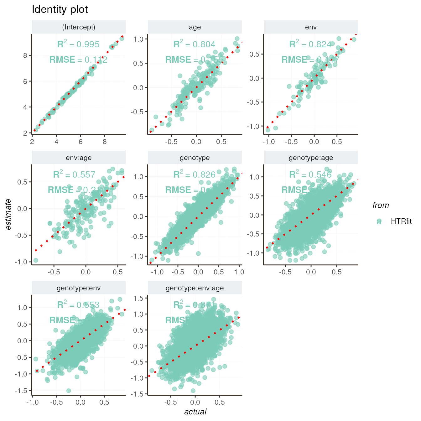
The metrics returned by evaluation_report() indicate
that capturing triple interactions is significantly more challenging
than main and simple interaction effects (between two variables). The
metrics comparing actual and inferred values are consistently lower for
triple interactions, as well as the classification metrics (AUC).
## -- actual/estimate comparison
resSimu$performances$byparams[c(2,4,6,5,7,8,9), c('description','R2', 'RMSE')]| description | R2 | RMSE |
|---|---|---|
| age | 0.8039539 | 0.1545807 |
| env | 0.8244036 | 0.1474956 |
| genotype | 0.8255563 | 0.1561758 |
| env:age | 0.5573628 | 0.2095237 |
| genotype:age | 0.5459986 | 0.2180452 |
| genotype:env | 0.5531829 | 0.2117465 |
| genotype:env:age | 0.3713272 | 0.2973623 |
## -- classification metrics
resSimu$performances$byparams[c(2,4,6,5,7,8,9), c('description',    'pr_AUC',
                                                  'pr_randm_AUC', 'pr_performance_ratio',
'roc_AUC', 'roc_randm_AUC')]| description | pr_AUC | pr_randm_AUC | pr_performance_ratio | roc_AUC | roc_randm_AUC |
|---|---|---|---|---|---|
| age | 0.8566991 | 0.5309278 | 1.613589 | 0.7874747 | 0.5 |
| env | 0.9047991 | 0.4329897 | 2.089655 | 0.8772727 | 0.5 |
| genotype | 0.8681321 | 0.5040882 | 1.722183 | 0.8228377 | 0.5 |
| env:age | 0.7205054 | 0.4278351 | 1.684073 | 0.7540975 | 0.5 |
| genotype:age | 0.6670356 | 0.3451831 | 1.932411 | 0.7331584 | 0.5 |
| genotype:env | 0.6832815 | 0.3537149 | 1.931730 | 0.7418028 | 0.5 |
| genotype:env:age | 0.5678086 | 0.3435834 | 1.652608 | 0.6646496 | 0.5 |
Improving triple interaction estimation
To improve the estimation of genotype:age:env triple
interaction, one strategy would be to increase the number of replicates
in our simulation. In this scenario, we use 25 replicates for each
experimental condition.
MIN_REPLICATES <- 25
MAX_REPLICATES <- 25

## -- simulate RNA-seq data
mock_data <- mock_rnaseq(input_var_list,
                         n_genes = N_GENES,
                         min_replicates  = MIN_REPLICATES,
                         max_replicates = MAX_REPLICATES,
                         basal_expression = PUB_BASAL_EXPR,
                         sequencing_depth = SEQ_DEPTH,
                         dispersion = DISP_PUB )
## -- prepare data
## apply + 1 to each counts
## remove genes i with all(k_ij) < 10
data2fit = prepareData2fit(countMatrix = mock_data$counts,
                           metadata =  mock_data$metadata,
                           normalization = 'MRN',
                           response_name = "kij",
                           transform = "x+1",
                           row_threshold = 10)

model2fit <- kij ~ genotype + env + age +
                   genotype:env + genotype:age + env:age +
                   genotype:age:env

## fit complex model
l_tmb <- fitModelParallel(
          formula = model2fit,
          data = data2fit,
          group_by = "geneID",
          family = glmmTMB::nbinom2(link = "log"),
          n.cores = 1,
          control = glmmTMB::glmmTMBControl(optCtrl=list(iter.max=1e5,
                                                         eval.max=1e5)))
## -- eval params for Wald test
ln_FC_threshold <- log(1.25) ## 25% of expression change
alternative_hypothesis <- "greaterAbs"
## -- remove genes with very low AIC
l_genes <- identifyTopFit(l_tmb)
## -- evaluation
resSimu <- evaluation_report( list_tmb = l_tmb,
                              list_gene = l_genes,
                              mock_obj = mock_data,
                              coeff_threshold = ln_FC_threshold,
                              alt_hypothesis = alternative_hypothesis )
We observe a significant improvement in performance across all
parameters, including the genotype:age:env parameter. The
inference of genotype:age:env is closer to the actual
values (R2, RMSE), and the model’s ability to determine whether a
parameter is differentially expressed or not (with a 25% expression
change) is enhanced (pr_AUC, ROC AUC).
## -- actual/estimate comparison
resSimu$performances$byparams[c(2,4,6,5,7,8,9), c('description','R2', 'RMSE')]| description | R2 | RMSE |
|---|---|---|
| age | 0.9691926 | 0.0777417 |
| env | 0.9396715 | 0.0790170 |
| genotype | 0.9566792 | 0.0682572 |
| env:age | 0.8336830 | 0.0945786 |
| genotype:age | 0.8741091 | 0.0873314 |
| genotype:env | 0.8313946 | 0.1030543 |
| genotype:env:age | 0.7410645 | 0.1319104 |
## -- classification metrics
resSimu$performances$byparams[c(2,4,6,5,7,8,9), c('description', 'pr_AUC',
                                                  'pr_randm_AUC', 'roc_AUC',
'roc_randm_AUC')]| description | pr_AUC | pr_randm_AUC | roc_AUC | roc_randm_AUC |
|---|---|---|---|---|
| age | 0.9466897 | 0.4642857 | 0.9242805 | 0.5 |
| env | 0.9768254 | 0.5102041 | 0.9566667 | 0.5 |
| genotype | 0.9503246 | 0.4982407 | 0.9137898 | 0.5 |
| env:age | 0.8753213 | 0.3112245 | 0.8646023 | 0.5 |
| genotype:age | 0.8596407 | 0.3446517 | 0.8397253 | 0.5 |
| genotype:env | 0.8480899 | 0.3427164 | 0.8391174 | 0.5 |
| genotype:env:age | 0.7951227 | 0.3335679 | 0.7947480 | 0.5 |
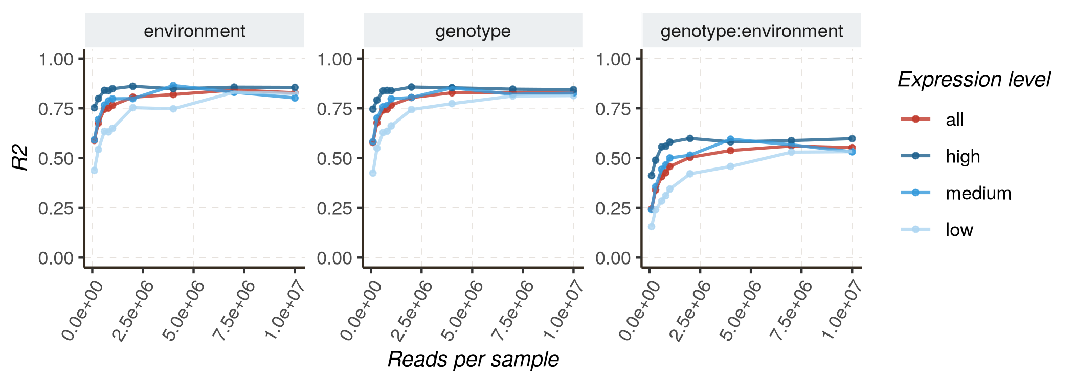
Examples of power analysis
HTRfit’s simulation framework offers flexibility in adjusting input parameters, enabling iterative monitoring of how biological or experimental parameters impact diverse performance metrics (ROC AUC, pr_AUC, R2, RMSE).
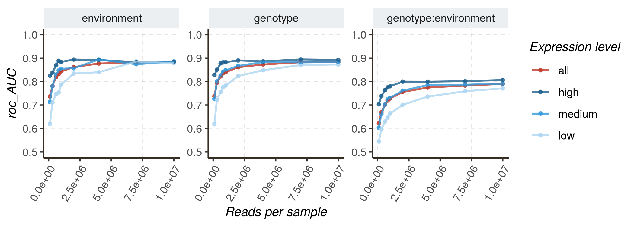
Monitoring results as sequencing depth increases
Increasing sequencing depth is expected to improve the model’s performance, either for the accuracy of parameter estimates (measured by R2 or RMSE) or for the quality of classification (distinguishing DE and non-DE genes, measured by AUC and PR_AUC). In this section, we utilize HTRfit to assess how model performances vary depending on sequencing depth. We perform this analysis for different groups of genes with different basal expression levels (low, medium, high). Indeed, we expect that model performances will be better for genes with higher expression levels.
- Fixed effects model :
kij ~ genotype + environment + genotype:environment
Follow these instructions to reproduce the graphs :


- Mixed effects model :
kij ~ environment + ( environment | genotype )
Similar graphs can be obtained for mixed effect model with these instructions.
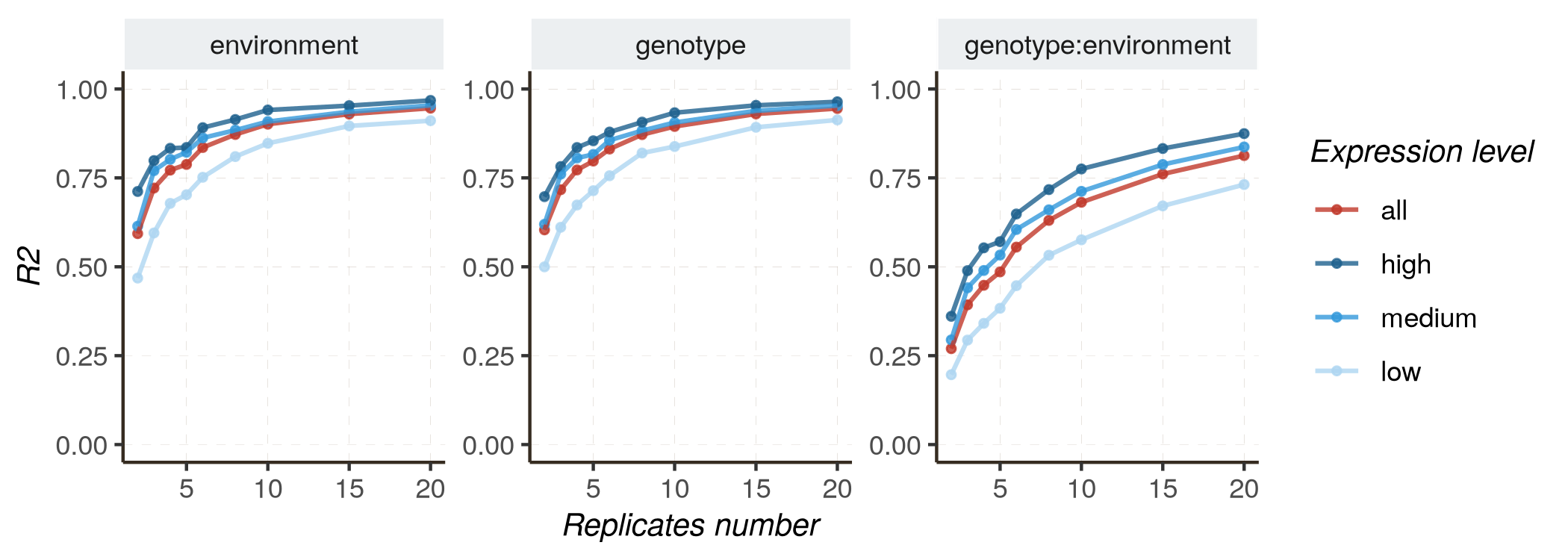
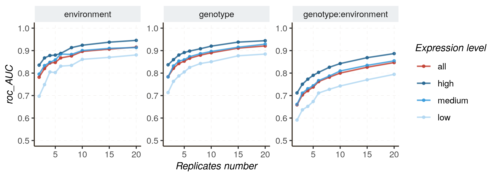
Monitoring results as replicates number increases
Increasing the number of replicates is also anticipated to improve performance, contributing to more accurate parameter estimation (measured by R2 or RMSE) and improved classification quality (distinguishing DE and non-DE genes, measured by AUC and PR_AUC).
- Fixed effects model :
kij ~ genotype + environment + genotype:environment
Follow these instructions to reproduce the graphs :


- Mixed effects model :
kij ~ environment + ( environment | genotype )
Similar graphs can be obtained for mixed effect model with these instructions.
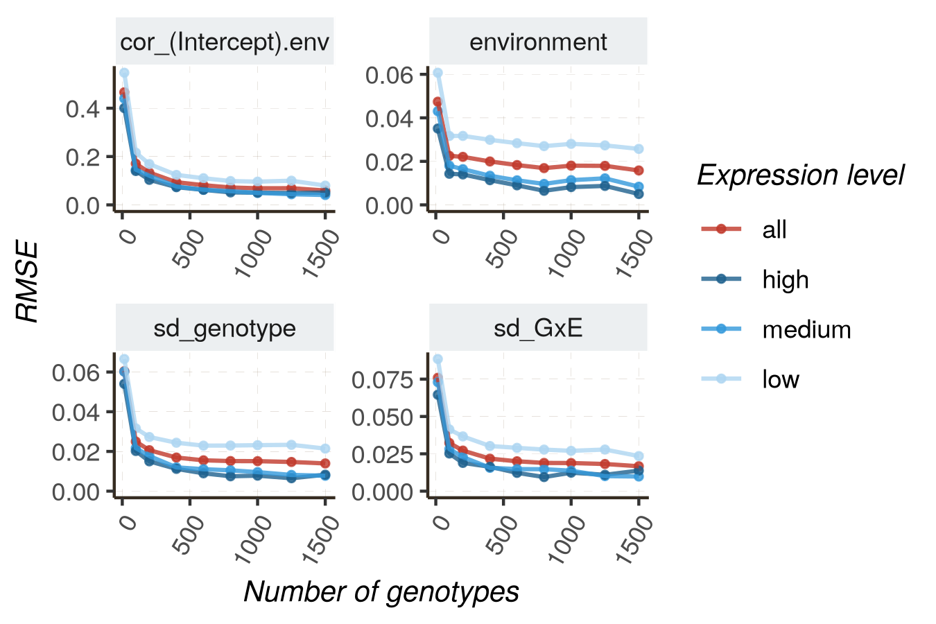
Monitoring accuracy in estimating random effect as number increases
To reproduce following graphs, follow these instructions
Grouping genes with different properties
Up to this point, during the simulation of mock RNA-seq data using
HTRfit, effect sizes (genotype, environment,
genotype:environment effects) were drawn from the same
distribution for all genes. With HTRfit’s combine_mock()
function, it becomes possible to generate intricate biological
experiments for which effect sizes are drawn from different normal
distributions for different groups of genes. This function allows the
user to simulate RNA-seq read counts for groups of genes with different
properties (for instance, genes that are sensitive to environmental
changes vs genes that are robust to environmental changes).
For further details about combine_mock() see object mock_rnaseq documentation
# N_GENES <- 100
SEQ_DEPTH <- mean(colSums(pub_data))/N_GENES
REP_NB <- 4
LIST_SD <- c(0.01, 0.04 , 0.07, 0.1, 0.13)

list_mock <- list()
for (SD in LIST_SD) {
  input_var_list <- init_variable(name = "genotype", sd = SD, level = 150) %>%
    init_variable(name = "env", sd = SD, level = 2) %>%
    add_interaction(between_var = c("genotype", "env"), sd =  SD)

  ## Use generate_counts = FALSE
  ## to save computing time and avoid generating something useless
  mock_data <- mock_rnaseq(
                  input_var_list,
                  n_genes = N_GENES/length(LIST_SD),
                  basal_expression = PUB_BASAL_EXPR,
                  dispersion = DISP_PUB,
                  generate_counts = FALSE)
  ## append new mock_data in a list
  list_mock <- append(list_mock , list(mock_data))
}

## -- counts are generated with combine_mock from the list_mock obj
mock_data <- combine_mock(list_mock, REP_NB, REP_NB, SEQ_DEPTH)
The capacity to merge genes with diverse behaviors into a unified
experiment proves especially beneficial when assessing a mixed model
(kij ~ environment + ( environment | genotype )) utilized
to infer sd(genotype) and sd(GxE). In such
instances, the identity plot generated by the
evaluation_report() will exhibit an R² for the random
effect (sd(genotype) and sd(GxE)) since the
actual value varies across genes.
## -- prepare data & fit model exactly as before
data2fit = prepareData2fit(countMatrix = mock_data$counts,
                           metadata =  mock_data$metadata,
                           normalization = 'MRN',
                           response_name = "kij",
                           transform = "x+1",
                           row_threshold = 10)
l_tmb <- fitModelParallel(
          formula = kij ~  env + ( env | genotype ) ,
          data = data2fit,
          group_by = "geneID",
          family = glmmTMB::nbinom2(link = "log"),
          n.cores = 1,
          control = glmmTMB::glmmTMBControl(optCtrl=list(iter.max=1e5,
                                                         eval.max=1e5)))
## -- eval params for Wald test
ln_FC_threshold <- log(1.25) ## 25% of expression change
alternative_hypothesis <- "greaterAbs"
## -- remove genes with very low AIC
l_genes <- identifyTopFit(l_tmb)
## -- evaluation
resSimu <- evaluation_report( list_tmb = l_tmb,
                              list_gene = l_genes,
                              mock_obj = mock_data,
                              coeff_threshold = ln_FC_threshold,
                              alt_hypothesis = alternative_hypothesis )
## -- Model params
resSimu$identity$params
## -- Model params
resSimu$violin_rand_params