RNA-seq analysis
03-rnaseq_analysis.RmdIn RNA-seq, we employ Generalized Linear Models (GLM) to unravel how genes respond to various experimental conditions. These models assist in deciphering the specific impacts of experimental variables on gene expression.HTRfit can be utilized to analyze such RNA-seq data, providing a robust framework for exploring and interpreting the intricate relationships between genes and experimental conditions.
Input data
HTRfit analysis necessitates a count matrix and sample metadata, in
the form of dataframes. Notice that gene_id have to be specified as
rownames of count_matrix. In this example we use
HTRfit to analyse a common RNA-seq data with 2
genotypes and 2 environments.
## -- gene count matrix
count_matrix[1:4, 1:2]
#>         genotype1_environment1_1 genotype1_environment1_2
#> gene1                         20                        6
#> gene10                         9                       15
#> gene100                       23                       24
#> gene11                        21                       20
## -- samples metadata
head(metaData)
#>    genotype  environment                 sampleID
#> 1 genotype1 environment1 genotype1_environment1_1
#> 2 genotype1 environment1 genotype1_environment1_2
#> 3 genotype1 environment1 genotype1_environment1_3
#> 4 genotype1 environment1 genotype1_environment1_4
#> 5 genotype1 environment2 genotype1_environment2_1
#> 6 genotype1 environment2 genotype1_environment2_2
Prepare data for fitting
The prepareData2fit() function serves the purpose of
converting the counts matrix and sample metadata into a dataframe that
is compatible with downstream HTRfit functions designed
for model fitting. This function also includes an option to perform
median ratio normalization and transformation on the data counts.
## -- convert counts matrix and samples metadatas in a data frame for fitting
data2fit = prepareData2fit(
             countMatrix = count_matrix,
             metadata =  metaData,
             normalization = NULL,
             response_name = "kij")


## -- median ratio normalization
data2fit = prepareData2fit(
             countMatrix = count_matrix,
             metadata =  metaData,
             normalization = 'MRN',
             response_name = "kij")

## -- apply + 1 transformation on each counts
data2fit = prepareData2fit(
             countMatrix = count_matrix,
             metadata =  metaData,
             normalization = 'MRN',
             transform = "x+1",
             response_name = "kij")
Fit model from your data
The fitModelParallel() function enables independent
model fitting for each gene. The number of threads used for this process
can be controlled by the n.cores parameter.
l_tmb <- fitModelParallel(
          formula = kij ~ genotype + environment  + genotype:environment,
          data = data2fit,
          group_by = "geneID",
          family = glmmTMB::nbinom2(link = "log"),
          n.cores = 1)
Use mixed effect in your model
HTRfit uses the glmmTMB functions for model fitting algorithms. This choice allows for the utilization of random effects within your formula design. For further details on how to specify your model, please refer to the mixed model documentation.
l_tmb <- fitModelParallel(
          formula = kij ~ genotype + ( 1 | environment ),
          data = data2fit,
          group_by = "geneID",
          family = glmmTMB::nbinom2(link = "log"),
          n.cores = 1)
Additional settings
The function provides precise control over model settings for fitting
optimization, including options for specifying the model
family and model
control setting. By default, a Gaussian family model is fitted, but
for RNA-seq data, it is highly recommended to specify
family = glmmTMB::nbinom2(link = "log").
l_tmb <- fitModelParallel(
          formula = kij ~ genotype + environment  + genotype:environment,
          data = data2fit,
          group_by = "geneID",
          n.cores = 1,
          family = glmmTMB::nbinom2(link = "log"),
          control = glmmTMB::glmmTMBControl(optCtrl=list(iter.max=1e5,
                                                         eval.max=1e5)))
Extracts a tidy result table from a list tmb object
The tidy_results function extracts a data frame containing estimates of ln(fold changes), standard errors, test statistics, p-values, and adjusted p-values for fixed effects. Additionally, it provides access to correlation terms and standard deviations for random effects, offering a detailed view of HTRfit modeling results.
## -- get tidy results
my_tidy_res <- tidy_results(l_tmb, coeff_threshold = 0.1,
                            alternative_hypothesis = "greaterAbs")
## -- head
my_tidy_res[1:3,]
#>      ID effect component group         term    estimate std.error   statistic
#> 1 gene1  fixed      cond    NA  (Intercept)  2.84081018 0.1209488  2.01401422
#> 2 gene1  fixed      cond    NA    genotype2 -0.02527887 0.1723802 -0.60539186
#> 3 gene1  fixed      cond    NA environment2  0.59941560 0.1504515 -0.06525054
#>         p.value         p.adj
#> 1 5.445603e-114 3.203296e-113
#> 2  9.013490e-01  9.268370e-01
#> 3  4.526502e-04  1.240138e-03
Update fit
The updateParallel() function updates and re-fits a
model for each gene. It offers options similar to those in
fitModelParallel(). In addition, it is possible to modify
the reference level of the categorical variable used in your model in
order to use different contrast.
## -- update your fit modifying the model family
l_tmb <- updateParallel(
          formula =  kij ~ genotype + environment  + genotype:environment,
          list_tmb = l_tmb ,
          family = gaussian(),
          n.cores = 1)

## -- update fit using additional model control settings
l_tmb <- updateParallel(
          formula =  kij ~ genotype + environment  + genotype:environment ,
          list_tmb = l_tmb ,
          family = gaussian(),
          n.cores = 1,
          control = glmmTMB::glmmTMBControl(optCtrl=list(iter.max=1e3,
                                                         eval.max=1e3)))


## -- update your model formula and your family model
l_tmb <- updateParallel(
            formula =   kij ~ genotype + environment  ,
            list_tmb = l_tmb ,
            family = glmmTMB::nbinom2(link = "log"),
            n.cores = 1)

## -- modif reference levels
## -- genotype reference = "genotype2"
## -- environment reference = "environment2"
l_tmb <- updateParallel(
            formula =   kij ~ genotype + environment  ,
            list_tmb = l_tmb ,
            family = glmmTMB::nbinom2(link = "log"),
            n.cores = 1,
            reference_labels = c("genotype2", "environment2"))
Struture of list tmb object
str(l_tmb$gene1, max.level = 1)
#> List of 8
#>  $ obj      :List of 10
#>  $ fit      :List of 7
#>  $ sdr      :List of 8
#>   ..- attr(*, "class")= chr "sdreport"
#>  $ call     : language glmmTMB::glmmTMB(formula = kij ~ genotype + environment, data = data, family = list(     family = "nbinom2", vari| __truncated__ ...
#>  $ frame    :'data.frame':   16 obs. of  5 variables:
#>  $ modelInfo:List of 15
#>  $ fitted   : NULL
#>  $ groupId  : chr "gene1"
#>  - attr(*, "class")= chr "glmmTMB"
Plot fit metrics
Visualizing fit metrics is essential for evaluating your models. Here, we show you how to generate various plots to assess the quality of your models. You can explore all metrics or focus on specific aspects like dispersion and log-likelihood.
## -- plot all metrics
diagnostic_plot(list_tmb = l_tmb)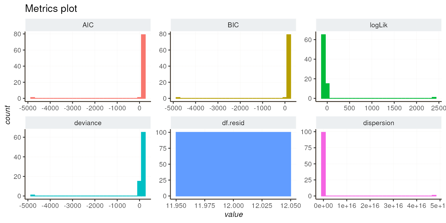
## -- Focus on metrics
diagnostic_plot(list_tmb = l_tmb, focus = c("AIC"))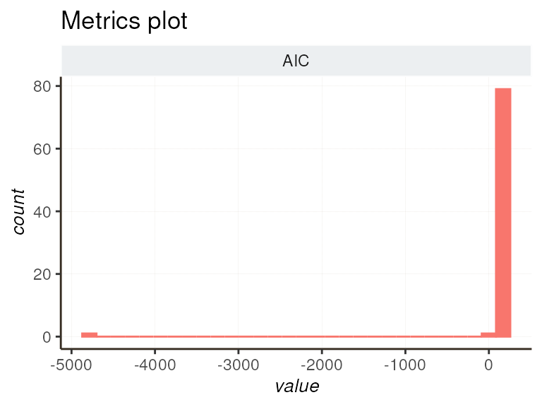
Select best fit based on diagnostic metrics
The identifyTopFit function allows for selecting genes that best fit
models, based on various metrics such as AIC, BIC, LogLik, deviance,
dispersion . This function provides the flexibility to employ multiple
filtering methods to identify genes most relevant for further analysis.
We implemented a filtering method based on the Median Absolute Deviation
(MAD). For example, using the MAD method with a tolerance threshold of
3, the function identifies genes whose metric values are greater (“top”)
or lower (“low”) than median(metric) - 3 * MAD(metric). The
keep option allows choosing whether to retain genes with metric values
above or below the MAD threshold.
identifyTopFit(list_tmb = l_tmb, metric = "AIC",
               filter_method = "mad", keep = "top",
               sort = TRUE, decreasing = TRUE,
               mad_tolerance = 3)
#> Based on the specified metric (AIC) and the MAD filtering method, the following selection criteria were applied:
#> 1. The MAD-based threshold for considering outliers was calculated.
#> 2. Values above the threshold were identified, threshold: 85.2207505555877
#> 3. Summary of selection:
#> - 79 out of 100 observations had values above the threshold for the AIC metric.
#>  [1] "gene28" "gene50" "gene98" "gene39" "gene94" "gene61" "gene95" "gene93"
#>  [9] "gene38" "gene68" "gene30" "gene1"  "gene70" "gene22" "gene17" "gene63"
#> [17] "gene46" "gene27" "gene64" "gene7"  "gene75" "gene62" "gene29" "gene13"
#> [25] "gene78" "gene79" "gene88" "gene77" "gene52" "gene21" "gene35" "gene16"
#> [33] "gene25" "gene42" "gene58" "gene55" "gene9"  "gene43" "gene14" "gene18"
#> [41] "gene44" "gene32" "gene54" "gene5"  "gene10" "gene37" "gene2"  "gene99"
#> [49] "gene8"  "gene60" "gene19" "gene72" "gene23" "gene90" "gene40" "gene83"
#> [57] "gene20" "gene45" "gene3"  "gene96" "gene81" "gene11" "gene76" "gene80"
#> [65] "gene31" "gene51" "gene15" "gene24" "gene12" "gene92" "gene89" "gene87"
#> [73] "gene86" "gene4"  "gene84" "gene26" "gene6"  "gene69" "gene53"
Anova to select the best model
Utilizing the anovaParallel() function enables you to
perform model selection by assessing the significance of the fixed
effects. You can also include additional parameters like type. For more
details, refer to car::Anova.
## -- update your fit modifying the model family
l_anova <- anovaParallel(list_tmb = l_tmb)

## -- additional settings
l_anova <- anovaParallel(list_tmb = l_tmb, type = "III" )